Preprocess Data MIPMLP (Mendatory)

Preproceesing the raw ASVs by the following steps:
 (1) merging similar features based on the taxonomy
 (2) scaling the distribution
 (3) standardization to z-scores (optional)
 (4) and dimension reduction (optional)

Input

- The input file for the preprocessing should contain detailed unnormalized OTU/Feature values as a biom table, the appropriate taxonomy as a tsv file.
- A merged otu and taxonomy csv, such that the first column is named "ID", each row represents a sample and each column represents an ASV. The last row contains the taxonomy information, named "taxonomy".

Here is an example of how the input OTU file should look like: example_file.csv.

Optional

 - It is possible to load a tag file, with the class of each sample.
 - The tag file is not used for the preprocessing, but is used to provide some statistics on the relation between the features and the class.
 - A tag file is mendatory for iMic, miMic, and for the visualization of SAMBA.
 - Note: One can also run the preprocessing without a tag file.

Here is an example of how the input TAG file should look like: example_file.csv.

Parameters

Select the parameters for the preprocessing.

- taxonomy level - Taxonomy sensitive dimension reduction by grouping the taxa at a given taxonomy level. All features with a given representation at a given taxonomy level will be grouped and merged using three different methods: Average, Sum or Sub-PCA (using PCA then followed by normalization).
Select one of: {"Order", "Family", "Genus", "Species"}. Default is "Species".

- Normalization - After the grouping process, you can apply two different normalization methods:
- Log (10 base) scale If you chose the log normalization, you now have four standardization:    a) No standardization
   b) Z-score each sample
   c) Z-score each bacteria
   d) Z-score each sample, and Z-score each bacteria (in this order)
- Relative scale ("Relative")
When performing relative normalization, we either do not standardize the results or preform only a standardization on the taxa.
Select one of: {"Log", "Relative"}. Default is "Log".

- Dimension Reduction - After the grouping, normalization and standardization you can choose from two dimension reduction method: "PCA" or "ICA".
Select one of: {"None","PCA","ICA"}. Default is "None".
- Note if you chose to apply a Dimension reduction method, you will also have to decide the number of dimensions you want to leave.

- Taxonomy Group - The method to merge different ASVs of the same taxonomy.
Select one of: {"sub PCA", "mean", "sum"}. Default is "sub PCA".

- sub PCA - A taxonomic level (e.g., species) is set. All the ASVs that are consistent with this taxonomy are grouped. A PCA (Principal component analysis) is performed on this group. The components that explain more than half of the variance are added to the new input table.
- mean - A level of taxonomy (e.g., species) is set. All the ASVS consistent with this taxonomy are grouped by averaging them.
- sum - A level of taxonomy (e.g., species) is set. All the ASVS consistent with this taxonomy are grouped by summing them.

- Epsilon - The pseudo index is added to the data to prevent zeros when "log normalization" is applied.
Select a number between 0 to 1. Default is 0.1.

- Number of components - If dimension reduction is not "None", select a number for reduction.
Select a number. Default is 0.

- Taxonomy level for frequency plot - For visualizations only.
Select one of: {"Class", "Phylum", "Order"}. Default is "Class".

- Z scoring following log normalization - How to apply z-scoring after the log normalization.
Select one of: {"None", "Row","Col","Both"}. Default is "None".

- Z scoring following relative frequency - How to apply z-scoring after the log normalization.
Select one of: {"No", "Row","Col","Both"}. Default is "No".

Output

The output is the processed file.

iMic (Optional)

Tick the box next to iMic to select.
iMic is a method to combine information from different taxa and improves data representation for machine learning using microbial taxonomy. iMic translates the microbiome to images by using a cladogram of means, and convolutional neural networks are then applied to the image.

Input

The same inputs as for the data preprocessing.

Parameters

Select the parameters for iMic running:
 - l1 loss = the coefficient of the L1 loss
 - weight decay = L2 regularization
 - lr = learning rate
 - batch size = as it sounds
 - activation = activation function one of: "elu", | "relu" | "tanh"
 - dropout = as it sounds (is common to all the layers)
 - kernel_size_a = the size of the kernel of the first CNN layer (rows)
 - kernel_size_b = the size of the kernel of the first CNN layer (columns)
 - stride = the stride's size of the first CNN
 - padding = the padding size of the first CNN layer
 - padding_2 = the padding size of the second CNN layer
 - kernel_size_a_2 = the size of the kernel of the second CNN layer (rows)
 - kernel_size_b_2 = the size of the kernel of the second CNN layer (columns)
 - stride_2 = the stride size of the second CNN
 - channels = number of channels of the first CNN layer
 - channels_2 = number of channels of the second CNN layer
 - linear_dim_divider_1 = the number to divide the original input size to get the number of neurons in the first FCN layer
 - linear_dim_divider_2 = the number to divide the original input size to get the number of neurons in the second FCN layer
 - input dim = the dimention of the input image (rows, columns)
Note that the input_dim is also updated automatically during the run.

Output

The train and test sets as csv files along with the model's AUC score for them.

miMic (Optional)

Tick the box next to miMic to select.
miMic is a straightforward yet remarkably versatile and scalable approach for differential abundance analysis.
miMic consists of three main steps:
 - Data preprocessing and translation to a cladogram of means.  - An apriori nested ANOVA (or nested GLM for continuous labels) to detect overall microbiome-label relations.  - A post hoc test along the cladogram trajectories.

Input

The same inputs as for the data preprocessing.

Parameters

Select the parameters for miMic running:
 - Eval Mode: evaluation method, ["man", "corr", "cat"]. Default is "man".
   - "man" for binary labels.
   - "corr" for continuous labels.
   - "cat" for categorical labels.
 - sis: apply sister correction,["fdr_bh", "bonferroni", "no"]. Default is "fdr_bh".
 - Correct First: apply FDR correction to the starting taxonomy level according to `sis` parameter,[True, False] Default is True.
 - p-value: the threshold for significant values. Default is 0.05.
 - THRESHOLD_edge: the threshold for having an edge in "interaction" plot. Default is 0.5.

Output

- corrs_df: a dataframe containing the results of the miMic test (including Utest results).

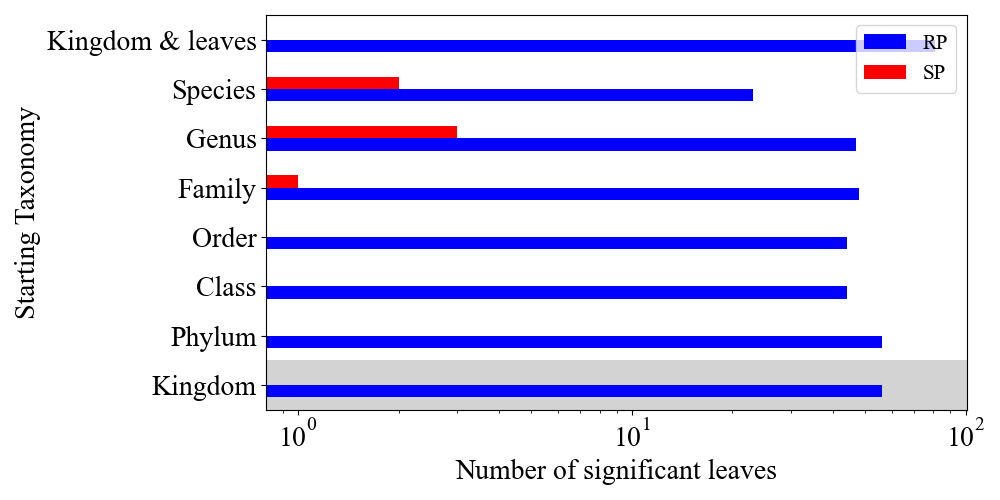
- tax_vs_rp_sp_anova_p: plot RP vs SP over the different taxonomy levels and color the background of the plot till the selected taxonomy, based on miMic test.



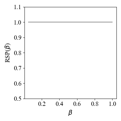
- rsp_vs_beta: calculate RSP score for different betas and create the appropriate plot.



- hist: a histogram of the ASVs in each taxonomy level.



- corrs_within_family: a plot of the correlation between the significant ASVs within the family level, the background color of the node will be colored based on the family color.



- interaction: a plot of the interaction between the significant ASVs.



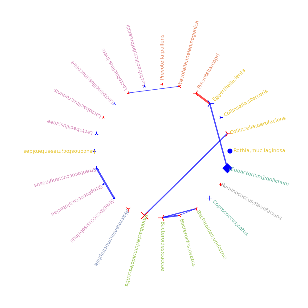
- correlations_tree: create correlation cladogram, such that tha size of each node is according to the -log(p-value), the color of each node represents the sign of the post hoc test, the shape of the node (circle, square,sphere) is based on miMic, Utest, or both results accordingly, the background color of the node will be colored based on the family color.

SAMBA (Optional)

Tick the box next to iMic to select.
SAMBA is a novel microbial metric. SAMBA utilizes the iMic method to transform microbial data into images, incorporating phylogenetic structure and abundance similarity. This image-based representation enhances data visualization and analysis. Moreover, SAMBA employs a fast Fourier transform (FFT) with adjustable thresholding to smooth the images, reducing noise and accentuating meaningful information. Various distance metrics, such as SAM and MSE, can be applied to the processed images.

Input

The same inputs as for the data preprocessing.

Parameters

Select the parameters for SAMBA running:
 - cutoff - A number between 0 to 1. Default is 0.8. It is the cutoff for the FFT filtering.
 - metric - The metric to calculate the distances between the created images.
Select one of {"sam","mse","d1","d2","d3"}.

Output

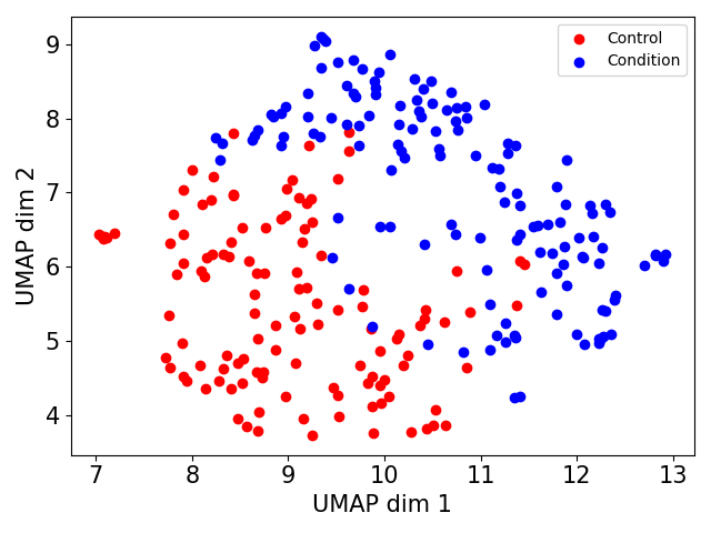
- A csv with SAMBA's distances matrix.
- If a tag file is provided, a 2D-UMAP visualization colored according to the tag file.

Cite US

- Shtossel, Oshrit, et al. "Ordering taxa in image convolution networks improves microbiome-based machine learning accuracy." Gut Microbes 15.1 (2023): 2224474.

- Shtossel, Oshrit, and Yoram Louzoun. "miMic-a novel multi-layer statistical test for microbiome disease." (2023).

- Jasner, Yoel, et al. "Microbiome preprocessing machine learning pipeline." Frontiers in Immunology 12 (2021): 677870.